SQL Fundamentals — The Queries That Cover Most of What You Need

SQL has been around since 1974. It has outlasted dozens of technologies that were supposed to replace it. Today it is the language behind almost every relational database — Oracle, SQL Server, PostgreSQL, MySQL, SQLite, SAP HANA — and understanding it is one of those skills that quietly pays off in almost every technical role.

This post covers the core of SQL — the statements and concepts that cover the vast majority of real-world queries. Not every edge case, not every dialect difference — the foundation that makes everything else make sense.

What SQL is

SQL — Structured Query Language — is the standard language for interacting with relational databases. It lets you retrieve, insert, update and delete data, and define the structure of the database itself.

SQL category	What it covers	Examples
DQL — Data Query Language	Reading data	SELECT
DML — Data Manipulation Language	Inserting, updating, deleting data	INSERT, UPDATE, DELETE
DDL — Data Definition Language	Defining tables and structure	CREATE, ALTER, DROP
DCL — Data Control Language	Permissions and access	GRANT, REVOKE

This post focuses on DQL — reading data with SELECT. That is what most people need most of the time, and it is the foundation for everything else.

The SELECT statement — where everything starts

Every SQL query that reads data starts with SELECT. The basic structure is always the same:

SELECT column1, column2

FROM table_name;

Let us use a real example. Say you have an Orders table:

order_id	customer_name	amount	status	country
1001	Rakesh Narayan	1249.99	confirmed	Finland
1002	Anna Korhonen	340.00	pending	Finland
1003	Marco Bianchi	875.50	confirmed	Italy
1004	Sophie Dupont	120.00	cancelled	France
1005	Lars Eriksson	2100.00	confirmed	Sweden

SELECT customer_name, amount

FROM orders;

Returns: the customer_name and amount columns for every row in the table.

SELECT *

FROM orders;

The asterisk * means all columns. Use it for exploration — avoid it in production queries where you should name only the columns you need.

WHERE — filtering rows

WHERE filters which rows are returned. Only rows where the condition is true are included.

SELECT customer_name, amount

FROM orders

WHERE status = ‘confirmed’;

Returns only the three confirmed orders — Rakesh, Marco, Lars.

Operator	Meaning	Example
=	Equal to	status = ‘confirmed’
!= or <>	Not equal to	status != ‘cancelled’
> / <	Greater / less than	amount > 1000
>= / <=	Greater or equal / less or equal	amount >= 340
BETWEEN	Within a range (inclusive)	amount BETWEEN 100 AND 1000
IN	Matches any value in a list	country IN (‘Finland’, ‘Sweden’)
LIKE	Pattern match — % is wildcard	customer_name LIKE ‘R%‘
IS NULL	Value is empty	delivery_date IS NULL
AND / OR	Combine multiple conditions	status = ‘confirmed’ AND amount > 500

SELECT customer_name, amount, country

FROM orders

WHERE status = ‘confirmed’

AND amount > 500;

Returns: Rakesh (1249.99) and Lars (2100.00) — confirmed orders over 500.

ORDER BY — sorting results

SELECT customer_name, amount

FROM orders

ORDER BY amount DESC;

Returns all orders sorted by amount, highest first. Use ASC for ascending (default), DESC for descending.

GROUP BY and aggregate functions

GROUP BY collapses rows that share a value into a single row, letting you calculate totals, counts and averages per group.

Function	What it returns	Example
COUNT(*)	Number of rows	COUNT(*) — count of orders
SUM(col)	Total of a numeric column	SUM(amount) — total order value
AVG(col)	Average of a numeric column	AVG(amount) — average order value
MAX(col)	Highest value	MAX(amount) — largest order
MIN(col)	Lowest value	MIN(amount) — smallest order

SELECT country,

COUNT(*) AS order_count,

SUM(amount) AS total_value

FROM orders

WHERE status != ‘cancelled’

GROUP BY country

ORDER BY total_value DESC;

This query returns: for each country, how many non-cancelled orders exist and their total value — sorted by value descending. A real reporting query.

💡 HAVING vs WHERE

WHERE filters rows before grouping. HAVING filters groups after aggregation. Example: HAVING SUM(amount) > 1000 — only return groups where the total is over 1000. You cannot use WHERE to filter on an aggregate — that is what HAVING is for.

JOIN — combining tables

Almost all real databases have data spread across multiple tables. JOIN is how you bring them together in a single query.

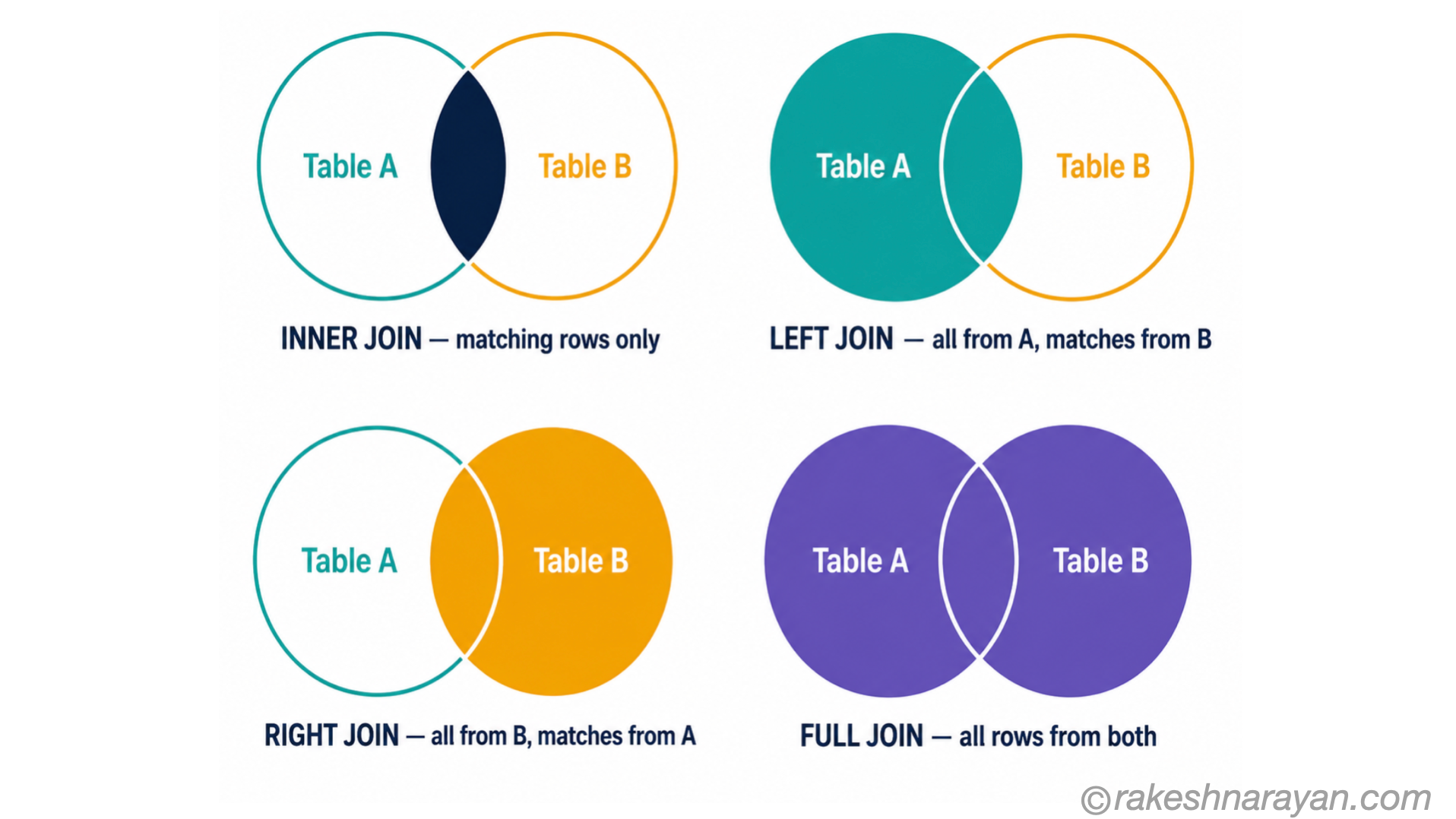
JOIN type	Returns	Most common?
INNER JOIN	Only rows with a match in both tables	Yes — the default in most queries
LEFT JOIN	All rows from the left table, plus matching rows from the right. NULL where no match.	Yes — common for optional relationships
RIGHT JOIN	All rows from the right table, plus matching rows from the left. NULL where no match.	Less common — LEFT JOIN with tables reversed is equivalent
FULL OUTER JOIN	All rows from both tables. NULL where no match on either side.	Rare — specific use cases

A practical JOIN example. Say you have a Customers table:

SELECT c.customer_name,

c.email,

o.amount,

o.status

FROM customers c

INNER JOIN orders o ON c.customer_id = o.customer_id

WHERE o.status = ‘confirmed’;

This returns customer name, email and confirmed order details — combining data from two tables via a shared customer_id.

Subqueries — queries inside queries

A subquery is a SELECT statement nested inside another query. It lets you use the result of one query as input to another.

SELECT customer_name, amount

FROM orders

WHERE amount > (

SELECT AVG(amount) FROM orders

);

Returns orders where the amount is above the average order value — without you having to calculate the average separately first.

SQL in the SAP context

SQL is not an abstract concept for SAP professionals — it shows up directly in daily work.

Where you encounter SQL in SAP	How it appears
ABAP Open SQL	ABAP’s SQL dialect for querying SAP tables — SELECT FROM BKPF WHERE BUKRS = ‘1000’
SAP HANA Studio / DBeaver	Direct SQL queries on HANA tables for analysis, debugging and data exploration
CDS Views	Core Data Services are SQL-based view definitions — the foundation of SAP Fiori and OData APIs
SAP Analytics Cloud	Custom calculations and dimensions often require SQL-like expressions
SAP Data Sphere	SAP’s data fabric platform uses SQL for data modelling and transformations
BTP Data Pipelines	SQL queries used in data flow tasks to transform and load data

💡 ABAP SQL vs standard SQL

ABAP Open SQL is a subset of standard SQL with SAP-specific syntax. Key differences: table and field names follow SAP naming conventions (MANDT, BUKRS), JOINs work but with some restrictions, and there is no GROUP BY in older ABAP — aggregates use LOOP AT instead. In S/4HANA, ABAP SQL has been extended significantly and CDS Views handle most complex query logic.

The SQL query execution order

This is something many people learn late and wish they had known earlier. SQL clauses are written in one order but executed in a different order.

Execution order	Clause	What it does
1	FROM / JOIN	Identify the source tables and combine them
2	WHERE	Filter rows before grouping
3	GROUP BY	Group rows by the specified column(s)
4	HAVING	Filter groups after aggregation
5	SELECT	Choose which columns to return
6	ORDER BY	Sort the final result
7	LIMIT / TOP	Restrict the number of rows returned

💡 Why this matters

You cannot use a SELECT alias in a WHERE clause — because WHERE is evaluated before SELECT. You cannot filter on an aggregate with WHERE — use HAVING because it runs after GROUP BY. Knowing the execution order explains most SQL errors instantly.

Quick reference — the core SQL

Statement / clause	Purpose	Key syntax
SELECT	Choose columns to return	SELECT col1, col2 FROM table
WHERE	Filter rows	WHERE amount > 500 AND status = ‘confirmed’
ORDER BY	Sort results	ORDER BY amount DESC
GROUP BY	Aggregate rows by a column	GROUP BY country
HAVING	Filter aggregated groups	HAVING SUM(amount) > 1000
INNER JOIN	Return matching rows from both tables	JOIN table2 ON table1.id = table2.id
LEFT JOIN	Return all rows from left table	LEFT JOIN table2 ON table1.id = table2.id
COUNT / SUM / AVG	Aggregate functions	SELECT COUNT(*), SUM(amount), AVG(amount)
LIKE	Pattern matching	WHERE name LIKE ‘R%‘
IN	Match against a list	WHERE country IN (‘FI’, ‘SE’, ‘IT’)
IS NULL	Check for empty values	WHERE delivery_date IS NULL
LIMIT / TOP	Restrict number of rows	LIMIT 10 (MySQL/PG) or TOP 10 (SQL Server)

What to take away

SQL is deceptively simple to start and genuinely deep to master. The fundamentals in this post — SELECT, WHERE, JOIN, GROUP BY and subqueries — cover the vast majority of what you will need for data exploration, integration work, report writing and system debugging.

In the SAP world specifically, ABAP SQL and CDS Views are built on these same foundations. Getting comfortable with standard SQL makes SAP’s data layer much easier to reason about.

🔗 Related posts on this site

JSON — From Zero to Confident — APIs return data in JSON; databases store the same data in tables. The two formats are complementary.
REST API Design Principles — REST APIs often expose data that is ultimately stored in and queried from relational databases.
SAP S/4HANA vs ECC — CDS Views, which are SQL-based, are central to the S/4HANA data model and Fiori app architecture.

Published on rakeshnarayan.com — Articles

URL: https://rakeshnarayan.com/articles/sql-fundamentals/